Definitions

Confounding factors

• The effect of two or more variables that do not allow a conclusion about either one separately. E.g: smoking study, do these participants also drink alcohol (confounding factor)?

Bias

• The systematic tendency of any factors associated with the design, conduct, analysis, and evaluation of the results of a trial to make the estimate of a treatment effect deviate from its true value.

Validity

• In logic, an argument is valid if the conclusions follow from the premises.
• In pharmaceutical science, a method is valid if it measures what it should, is reproducible, and responsive to change, for example by a treatment.

Dependent Vs. Independent Variables

• A variable is any data point that can be measured. E.g: BP, pain, age, death, stroke, SCr.
• Dependent variable (DV): "depends" on the intervention. E.g: compare atorvastatin versus placebo to see if atorvastatin has an impact on the number of secondary CVD events. The dependent variable (outcome) is the number of secondary CVD events.
• Independent variable (IV): is the intervention that the researchers manipulate, in order to determine whether it has an effect on the DV (outcome). In the example above, the independent variable is atorvastatin.

Incidence Vs. Prevalence

• Incidence: number of new cases of a disease per population at risk during a specific period. E.g: new cases per 1000 at-risk people per year, the incidence of hypertension (# of new cases) is 12105 per year within the Northeast region of the US.
• Prevalence: the total number of cases in a population found to have a condition in a given period of time. E.g., the prevalence of hypertension is 15% of the US population in 2011.

 

Types of data

Continuous data

• Logical order with values increases or decreases by the same amount. Two types: interval data, ratio data.
• Interval data: no meaningful zero, e.g.: temperature scale (0^o C = freezing point of water); Ratio data: has a meaningful zero (0=none). E.g.: HR = 0, means the heart is not beating; age, height, weight, BP.

Discrete (categorical) data

• Two types: nominal and ordinal data.
• Nominal data: synonymous with categorical data, where data is simply assigned “names” or categories based on attributes/characteristics, no ranking. For example: males/females; by religion as Hindu, Muslim, or Christian.
• Ordinal data: It is also called as ordered, or graded data (scores or ranks). For example, pain scale, heart failure stages.

Central tendency

• How do we provide a simple overview of the data? The descriptive values including the mean, median, and mode measure the central tendency,
• Mean: the average of a data set; preferred for continuous data in the normal distribution.
  • Mean = sum of all values / (n) values
• Median: value that sits in the middle of a set of ordered data (arranged from lowest to highest).
  • 50% of the population has a value smaller than the median, and 50% of samples values are larger than the median.
  • In the case of even numbers taken by an average of 2 middle values; and in the case of an odd number, the central value is the median.
  • Median is preferred for ordinal or continuous data that is skewed, a better indicator of central value when the lowest or the highest observations are wide apart.
• Mode: the number that occurs most often within a set of numbers, preferred for nominal data.
  • A dataset can have more than 1 mode. If no number in a set of numbers occurs more than once, that set has no mode.
• Practice: NAPLEX scores for 10 students are: 75, 82, 90, 92, 67, 95, 110, 80, 82, 86. Find the mean, median, mode for the above data.
  • First, arrange the set in order: 67, 75, 80, 82, 82, 86, 90, 92, 95, 110
  • Mean = (67+….+110)/10 = 85.90
  • Median = (82+86)/2 = 84
  • Mode= 82

 

Variability (spread) of Data

• Two common methods: the range and standard deviations (σ), measures the variability (how spread out your data is); Think like "variation" or "dispersion."
• Range: the difference between the lowest and highest values.
• Standard deviations (SD): shows how spread out the data is, and to what degree it is spread out over a smaller or larger range. A small SD means data is tightly clustered around the mean. Inversely, a large SD means data is highly dispersed. 
• The SD provides value when the sample is normally distributed and is used for continuous variables. SD would not be appropriate to measure bimodal or skewed data.

 

Distribution

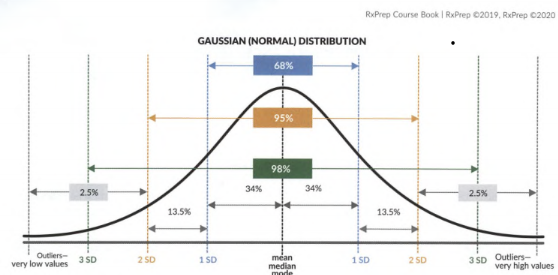
• Normal (AKA parametric, Gaussian) distribution is a bell-shaped graph and symmetrical (even on both sides); at the apex: mean = median = mode (however this would not be the case for skewed data). A small number of values are in the tails.
• 68% of data falls within +/- 1 SD, 95% within +/- 2 SD, 99.7% values within +/- 3 DS of the mean.

• Skewed (non-parametric): non-symmetrical. This is usually the case when the sample size is small or there are outliers in the data. Skew refers to the direction of the tail, not the bulky hump. 

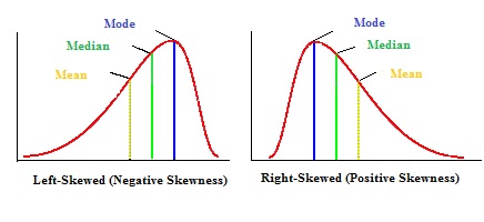
• Outliers are extreme values, either very low or very high. They can have a large impact on the mean (averaging the dataset). The distortion of the central tendency by outliers can be reduced by collecting more data.
• The median value is a better predictor of central tendency in skewed data, and interquartile range (IQR) is a better predictor of variability than SD.

Testing the hypothesis for statistical significance

Research data can demonstrate whether a drug or device is significantly better than the current treatment or a placebo. In order to show significance, trials need to show that the null hypothesis is not true (be rejected), and the alternative hypothesis is accepted.

Null Hypothesis (H0)

• No statistically significant difference between groups (drug efficacy = placebo). Researchers try to disprove or reject H₀. g: paroxetine is no better than a placebo at treating depression.

Alternative Hypothesis (H_A)

• A statistically significant difference (or relationship) exists between groups. E.g: paroxetine is statistically superior to placebo at treating depression. Researchers try to prove or accept H_A.

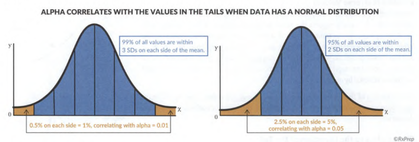
Alpha (α)

• the max permissible error margin selected by investigators when designing a study.
• It is the standard for significance and the threshold in rejecting the null hypothesis. Alpha is usually set at 0.05 (or 5%) in medical research. A smaller alpha requires more data (subjects) to reach a higher level of precision.

 

Confidence Interval (CI)

• provides the same info as the p-value plus the precision of the result. It is an estimate of the range where the true effect lies. CI = 1- α.
• If α = 0.05, CI corresponds to a 95% confidence interval (typical). The only way to have a 100% confidence interval is to measure the entire treatment population, which is unpractical and impossible.
• g., A study reports that patients taking a new diet drug for 90 days lose 10 kg, with a 95% confidence interval of 6 kg - 16 kg, which means they are 95% confident that anyone who takes this drug for 90 days will lose between 6 and 16 kg, so there is a 5% uncertainty.
• A narrow CI range implies high precision, and a wide CI implies poor precision. E.g.: You are 95% confident that the true value of the ARR lies within 6-35%, if the true value is between 4-68%, the range is wider and less precise.
• Compare difference data (means): the result is statistically significant if the CI range doesn’t include zero. E.g.: the 95% CI for FEV1 between roflumilast and placebo (18-58ml) doesn’t include zero: the result is statistically significant; the 95% CI for FEV1/FVC (-0.26 – 0.89) include zero -> the result is not statistically significant.
• Compare ratio data (relative risk, odds ratio, hazard ratio), the result is statistically significant if the CI range doesn’t include one.
• Ratio data: based on division. E.g., the ratio of severe exacerbation between roflumilast and placebo was 0.9 (=0.11/0/12)
• the 95% CI for the relative risk (0.72 – 0.99) is statistically significant, but the 95% CI for the relative risk (0.62 – 1.29) is not statistically significant (includes 1).

 

Type I & Type II Error

• Type I error ("false positive" or α error): Null hypothesis is true but was rejected in error. g: "This drug has an effect!" when it actually does not. The risk of making a type I error is determined by alpha and related to the CI.
  • If p-value < 0.05, there is < 5% chance to falsely reject a true null hypothesis.
• Type II error ("false negative" or β error): Null hypothesis is false but was accepted in error. There is a difference between groups, but the researchers say there is none.
  • Type II is related to power. Errors happen frequently in trials if not enough patients are enrolled. 
  • Knack: you want to be positive first and negative second. (Be positive!)

p-value

• Once the alpha value is determined, a p-value is calculated and compared to alpha. (Related to Type I Error).
• p < 0.05: the finding is statistically significant. The null hypothesis is rejected.
• p >/= 0.05: the finding is not statistically significant. The study has failed to reject the null hypothesis.

Statistical Power

• Ability to detect a significant difference between treatment groups. (Related to Type II Error).
• The conventional setting for statistical power is 80%. E.g: a study is powered at 80%, which means a 20% chance of committing Type II Error; power = 90%, only a 10% chance of Type II Error. 
• Increase the sample size will increase statistical power. The larger the sample size, the less chance of committing type II error.

 

Relative risk (RR or risk ratio)

• The risk of an event when an intervention (drug, or treatment) is given. 𝑅𝑅 = risk 𝑖𝑛 the 𝑖𝑛𝑡𝑒𝑟𝑣𝑒𝑛𝑡𝑖𝑜𝑛 𝑔𝑟𝑜𝑢𝑝 /risk 𝑖𝑛 the 𝑐𝑜𝑛𝑡𝑟𝑜𝑙 𝑔𝑟𝑜𝑢𝑝.
• E.g., the risk of heart attack in patients taking a study drug versus a control group of patients taking a placebo. The relative risk = Heart attacks rate in the intervention group / Heart attacks rate in the control group.
  • RR = 1: no difference between the groups; no association between exposure to a factor and the outcome of interest.
  • RR < 1: implies lower risk in the treatment group. 0.55 = the risk of heart failure was less with the study drug than the placebo, e.g., SGLT inhibitors from DM.
  • RR > 1: implies greater risk in the treatment group. 1.5 = the risk of heart failure is higher with the study drug than the placebo, e.g: TZD from DM.
• Practice: the event of heart attacks in the intervention group with drug X was 5 out of 100 patients, and the event of heart attacks in the control group with placebo was 9 out of 100 patients. RR = 0.05/0.09 = 0.55, X-treated patients were 55% as likely (as the control group) to develop heart attacks.

 

Relative risk reduction (RRR) Vs. Absolute risk reduction (ARR)

• The relative risk reduction (RRR) measures how much the treatment reduced the risk of an outcome (relative to the control group).
  • RRR = 1 - Relative Risk (RR)
  • Above example RRR = 1- 0.55 = 0.45: X-treated patients were 45% less likely to have heart attacks than placebo-treated patients.
• ARR: absolute difference of the event rate between the groups.
  • ARR = the event rate in the control group – the event rate in the intervention group
  • Practice: heart attack rate in the intervention group with drug X is 5%, and the rate in the placebo group is 9%. ARR = 9% - 5% = 4%: 4 out of 100 patients benefit from the treatment, or 4 fewer patients have heart attack.

 

Number needed to treat (NNT) or harm (NNH)

• An important clinical question can be answered: how many patients need to receive the drug for one patient to benefit (NNT) or harm (NNH)?
• NNT: Number of patients need to be treated to benefit one patient.
• 𝑁𝑁𝑇 = 1/𝐴𝑅𝑅, always round up to the nearest integer (avoid overstating the benefit) e.g., 11.2 would be rounded up to 12).
• Practice: heart attack rate in the intervention group with drug X is 2%, and the rate in the placebo group is 7%. ARR = 7% - 2% = 5%, NNT = 1/5% = 20, means for every 20 patients treated, heart attack can be avoided in 1 patient.
• NNH: Number of patients must be exposed (to a risk factor) to cause harm in one patient.
• NNH = 1/ ARI, always rounded down (avoids understanding the potential harm). E.g., NNH of 41.9 -> 41.
• Absolute risk increase (ARI) = difference between event rates in groups, similar to ARR (reduction), use larger number minus smaller number.
• Practice: myopathy rate in patients with heart failure taking statins was 5 out of 100, and among patients not taking statins, was 2 out of 100, calculate the relative risk.
  • RR = 0.05/0.02=2.5
  • ARI = 5% - 2% = 3%
  • NNH = 1/0.03 = 33.33 (one additional case of myopathy is expected to occur for every 33 patients taking statins instead of placebo).

 

Odds ratio (OR)

• Odds are the probability of an event will occur, versus the probability that it will not occur.
• Similar to RR, but it is used to estimate the risks in case studies, which are not suitable for RR. Case-control studies enroll patients who have an outcome already occurred (e.g., breast cancer) and are reviewed retrospectively to search for exposure risk. Therefore, OR is used to calculate the odds of an event occurring with an exposure, compared to the odds occurring without exposure.
• The formula is a bit crazy and shouldn’t be required for the exam: OR=(a/c)/(b/d)=ad/bc.

• a = exposed cases; b = exposed non-cases; c = unexposed cases; d = unexposed non-cases

• Different than RR: RR compares risks in 2 groups, OR compares the odds in 2 groups (ratio of two different sets of odds).

• Risk = [The chance of an outcome of interest] / [All possible outcomes]
• Odds = [Probability of event to occur] / [Probability of event not occurring] 

• g., A group of 100 smokers, 35 of them develop lung cancer, and that 65 do not. 

• The risk of lung cancer is 35 /100 = 0.35 = 35%
• The odds of lung cancer are 35 / 65 = 0.54 = 54%

• Odds ratios can determine whether a particular exposure is a risk factor and can compare the magnitude of risk factors.

 

Hazard ratio

• Hazard rate (HR): an unfavorable event occurs within a short period of time. It calculates the ratio between the treatment and control group.
• HR = HR in the treatment group / HR in the control group
• g. Niacin is evaluated whether it reduces CV risk. Primary endpoint (stroke, MI, death). Niacin hazard 282/1718 = 0.16, Control: 274/1696 = 0/16. HR = 0.16/0.16 = 1.
• Conclusion: there’s no benefit when adding niacin to statin therapy.
• OR (or HR) =1 Exposure does not affect the odds of the outcome
• OR (or HR) >1 Exposure associated with higher odds of the outcome. E.g., OR = 1.23 could mean serotonergic antidepressants are associated with a 23% increased risk of falls.
• OR (or HR) <1 Exposure associated with lower odds of the outcome

 

Correlation & regression

• Pearson correlation coefficient ("r"): how strong the relationship is between data. From 1 to -1.

• Spearman’s rank-order correlation (Rho): test correlation for ordinal, ranked data.
• Correlation determines the relationship between variables, if one variable changes, another variable would increase or decrease. However, correlation does NOT prove a causal relationship (# of hospital days does not cause infection)!
• 1: strongly positive correlation. When the IV (duration of hospital stay) causes the DV (infections) to ↑.
• -1: strongly negative correlation. When the IV causes the DV to ↓.
• 0: no correlation.
• Regression: describe the relationship between a DV and more than one IV. E.g., how much the value of the DV changes when the IVs change. It is common in observational studies (researchers evaluable multiple IVs or control for many confounding factors. 3 types of regressions: l) linear, for continuous data, 2) logistic, for categorical data, and 3) Cox regression, for categorical data in survival analysis.

 

Sensitivity and specificity

• Being able to evaluate these two metrics is important in answering questions regarding the validity of lab or diagnostic tests, “If the test is positive, what is the probability of having the disease?” “If the test is negative, what is the probability of not having the disease?”
• Sensitivity (the true positive): how effectively the test identifies patients with the condition. The higher the sensitivity, the better; a test with 100% sensitivity will be positive in all patients with the condition. Sensitivity is calculated from those who test positive out of those who actually have the condition ("true-positive" results%).
• Specificity ("true-negative"): how effectively a test identifies patients without the condition. The higher the specificity the better.

 

Chose the right statistical test

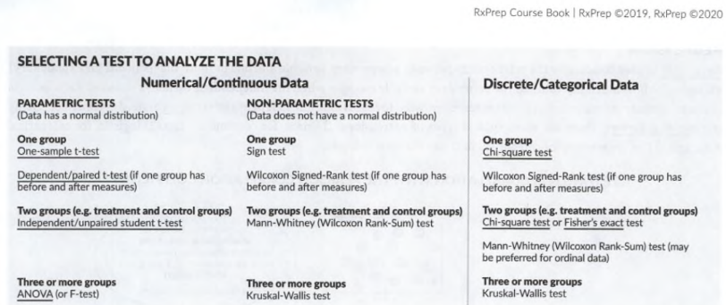
• Key questions to narrow down your choices: What type of data is it (Discrete or continuous)? Is the data parametric or skewed? How many study groups are there?
• T-tests (T = Two)
  • For continuous data with normal distribution.
  • One sample t-test: data from a single group is compared with known data from the general population.
  • Student t-tests (unpaired/independent) compare values of 2 independent groups. g., reduction in A1C between metformin and placebo.
  • paired t-test: compare before and after in the same group, e.g: measure a group of people’s weights at baseline and at 6 weeks. pre-/post- measurements use patients as their own control.
• ANOVA (analysis of variance, or F-test)
• Test statistical significance in continuous data with >= 3 groups.
• Similar to T-test: compare the distribution of a continuous variable. The distinction is that t-test can only be used to analyze 2 groups, ANOVA is 3+ groups.
• Can tell whether there is a statistical difference between groups but won’t tell you what that difference is. There is a power ball winner, but we don’t know who that is, can run a “post hoc” test to find out who that is.
• Repeated ANOVA: Test >3 dependent groups (e.g: effects of drug A, B, C at weeks 2, 6, and 10.)
• Discrete (categorical) data
• Chi-Square Test: Test statistical significance between groups for nominal or ordinal data. E.g., assess the difference between 2 groups in mortality (nominal data), or pain scores (ordinal).
• The only time you cannot use chi-square: to compare before and after measurements of the same population (use paired t-test).
• Non-parametric tests (not normally distributed, skewed data)
• tend to have fancy names: "Kruskal-Wallis," "Wilcoxon," and "Mann-Whitney U." 
• No means. If you are asked to compare the means of 2 populations and asked which test is appropriate, those law firm names are not the correct answers.


 

Data analysis in clinical trials

• 2 ways: intention-to-treat or per protocol.
• The intention-to-treat analysis includes data for all patients originally allocated to each group (treatment and control) even if the patient did not complete the trial (e.g., non-compliance, protocol violations, or withdrawal). This method is a conservative (real world) estimate of the treatment effect.
• Per protocol analysis: trial population who completed the study (or at least without any major protocol violations). This method provides an optimistic estimate of the treatment effect.

 

Trial design

• The standard design is to establish that treatment is superior to another treatment; the researcher wishes to show that the new drug is better than the old drug, or a placebo (less expensive, or toxic). Researchers would hope to demonstrate that the new drug is roughly equivalent (or at least not inferior) to the standard of care.
• Two types of trials: equivalence and non-inferiority trials.
• Equivalence trials attempt to show that the new treatment has about the same effect as the standard of care. Tests in 2 directions, for higher or lower effectiveness. (two-way margin).
• Non-inferiority trials: the new treatment is not worse. Test for effect in one direction (one-way margin).

 

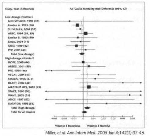
Forest plots and confidence intervals (CI)

• Forest plots: graphs with a “forest” of lines. Used either for multiple studies (results are pooled into a single study such as meta-analysis) or a single study (individual endpoints are pooled into a composite endpoint).
• Forest plots provide CIs for difference data or ratio data and help identify whether a statistically significant benefit has been reached.
• The boxes show the effect estimate. In a meta-analysis, the size of the box correlates with the size of the effect from the single study shown. Diamonds represent pooled results from multiple studies. 
• The horizontal lines through the boxes: length of the CI for that particular endpoint (single study) or in a meta-analysis. The longer the line, the wider the interval, and the less reliable the results. The width of the diamond in a meta-analysis serves the same purpose. 
• The vertical solid line is the line of no effect. A significant benefit has been reached when data falls to the left of the line; data to the right indicates significant harm. The vertical line is set at 0 for difference data and at 1 for ratio data. 
• Comparing difference data: in the meta-analysis by Miller et al. (Fig 1) a result is not statistically significant if the confidence interval crosses zero, so the vertical line (line of no difference), is set at zero. Examples: high-dosage vitamin E PPS shows a statistically significant benefit (the data point plus the entire CI, is to the left of the vertical line and does not cross 0). CHAOS: the result is not statistically significant (crosses 0). WAVE shows a statistically significant harmful outcome. 

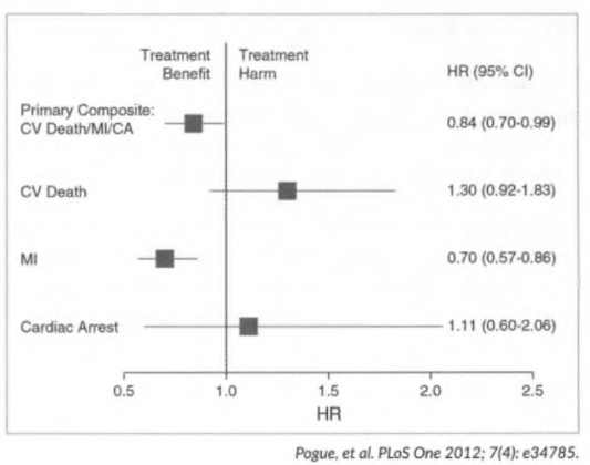
• Comparing ratio data: Fig 2 (by Pogue et al.) tests for significance of a composite endpoint in ratio data (in this case hazard ratio). For ratio data, the result is not statistically significant if the confidence interval crosses 1.  The primary composite endpoint shows a statistically significant benefit with treatment (Cl (0.7 - 0.99) does not cross 1). CV death: shows no statistically significant benefit/harm, the Cl (0.92 -1.8 3 ) crosses 1 (the horizontal line representing the Cl).


 

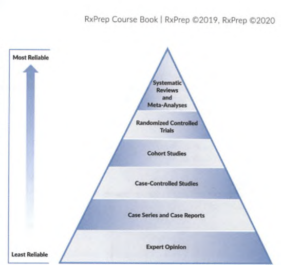
Types of research

• Evidence-based medicine (EBM) is the foundation of medical practice and most patient care recommendations and is largely guideline and protocol-driven.
• Case-control studies: retrospective; compare cases (patients with a disease) to controls (without a disease). Exam retrospectively to see if a relationship exists between the disease and risk factors. Benefits: easy to collect data from medical records. Suitable for unethical interventions but cannot determine cause and effect reliably (must use RCT).
• Cohort studies: compare exposure to those without exposure. Follow groups prospectively (or retrospectively, less common). Suitable for unethical interventions, but time-consuming and expensive than a retrospective study. Can be influenced by confounders (e.g., smoking, lipid levels).
• Cross-sectional survey: Estimates the relationship between variables and outcomes (prevalence) at one particular time (cross-section) in a defined population. Can identify associations (hypothesis-generating) for further studying but does not determine causality.
• CASE report and series: Describes an adverse reaction or a unique condition that appears in a single patient (case report) or a few patients (case series). Can identify new diseases, drug side effects, or potential uses. Generates hypotheses that can be further studied. Limitations: cannot draw conclusions from a single or few cases. E.g., A psychiatrist identified 2 cases of patients at his center who experienced the adverse effect, wrote it up, and published it in a medical journal.
• Randomized controlled trials (RCT): compare randomly assigned groups (treatment vs. placebo). Can determine cause and effect, or superiority. Less potential for bias. Limitations: Time-consuming and expensive. May not reflect real-life scenarios with rigorous exclusion criteria. Ex. Patients with HF were randomized in a double-blind manner to receive a new drug (ARNI) or the current standard of care (ACEI). The effectiveness of the treatments was measured as a primary composite outcome of death from CV causes or hospitalization for heart failure.
• Meta-analyses: analyzes the results of multiple studies. Prospective. E.g., The authors searched the PubMed database to locate studies investigating the use of antioxidants in people with CKD. Ten studies were identified, and the results were collected to try and identify whether antioxidants had an effect on cardiovascular disease and mortality in patients with CKD.


 

Pharmacoeconomics (FYI)

• Generally speaking, it is less of a focus for the NAPLEX scope. In order to direct your attention to the major pharmacotherapeutic areas, please read on your own for this topic, including the methodologies used to measure and compares the costs and consequences of pharmacotherapies and services.

 

Quiz

1. The median value of a data set is the

	A.		Average value of all the values in the data set.
	B.		value that is equal distance from both ends of a distribution.
	C.		average of the difference between each value in the set and the mean.
	D.		most commonly occurring number in the data set.
	E.		distance between the smallest and largest values in the data set.

 

• A study reports that the mean ± SD peak plasma concentration of a drug is 1.0 ± 0.2 mg/dL in a study consisting of 1,000 patients. Approximately how many patients had values >1.2 mg/dL?
1. 160
2. 680
3. 16
4. 840
5. 320

 

3.In a clinical study, and serum glucose concentrations were measured in 15 diabetic patients following 2 weeks of an investigational treatment to directly compare it to the decrease following glipizide treatment in a crossover trial. Statistics were performed and a p-value of 0.25 was obtained. Which of the following is the most likely statistical error that the researchers could have made?

1. Type I error
2. Type II error
3. Type I or type II error could not be made because the results were not significant
4. Type I or type II error could not be made because the results were significant

 

• In most clinical trials, Type I error rate is set to 0.05. This indicates that the researchers have a 5% chance of committing a Type I error. If the researchers were to set α at 0.02, corresponding to a Type 1 error rate of only 2%, which of the following statements is true?
  1. A smaller sample size could be used.
  2. The study power would increase.
  3. A possible increase of type I error
  4. A possible increase of type II error rate.
  5. None of the above statements is true.

 

5.What is the number needed to treat if drug A decreases the risk of myocardial infarction by 10% over drug B?

1. A.1
2. B.5
3. C.10
4. D.100
5. E.500

 

6. A study is conducted to assess the safety and efficacy of ketamine-propofol (KP) versus ketamine-dexmedetomidine (KD) for sedation in patients after CABG surgery. An appropriate test would be? If the trial added a third group, what test would be used? (The endpoint of fentanyl dose in KD 41.94+/- 20.43, KP 1542.8+/-51.2; Weaning/extubation time, min in KD 374.05 ± 20.25 KP 445.23 ± 21.7)

1. unpaired student t-test
2. Paired t-test
3. ANOVA
4. Chi-Square Test
5. Kruskal-Wallis

 

7. An emergency medical team wants to see if there is a statistically significant difference in death due to multiple drug overdose (OD) with at least one opioid taken, versus no opioid taken. Which test can determine a statistically significant difference in death? The endpoint of death in the opioid group is 20.8% and in the non-opioid group is 23.3%.

1. unpaired student t-test
2. Paired t-test
3. ANOVA
4. Chi-Square Test

 

• 8. Lab tests cyclic citrulline peptide (CCP) and rheumatoid factor (RF) are used in the diagnosis of rheumatoid arthritis (RA). Based on the table, what are the Sensitivity and Specificity for each test? If an elderly patient with swollen finger joints is referred to a rheumatologist and lab tests reveal a positive CCP and a positive RF, can a rheumatologist conclude that the patient has RA? Yes/No. If the RF is positive and the CCP is negative, what would be the rheumatologist’s conclusion and recommendation? can a rheumatologist conclude that the patient has RA? Yes/No.  

  CCP	Have RA	No RA	RF	Have RA	No RA
  +	A = 147	B = 9	+	A = 21	B = 26
  -	C = 3	D = 441	-	C = 54	D = 174
  Total	A+C = 150	B+D = 450	Total	A+C = 75	B+D = 200

 

9. Identify the appropriate studies being used.

• Data was pulled from 35 hospitals for all patients who had LEB during a 3-year period. Cases of surgical site infection (SSI) were identified and compared to those who did not develop an SSI (controls). An odds ratio (OR) was calculated for various risk factors that might increase SSI risk. ___
• Patients with type 1 DM who were taking statins (exposed) were compared to those not taking statins (not exposed) and followed for 7-12 years to see if statin use was associated with cognitive impairment (outcome). ___
• An analysis of 250 elderly women from August 2010 to April 2015 was performed. Data were collected retrospectively for 2 groups: SSRI users and nonusers to compare the prevalence of low BMD. No difference in the prevalence of low BMD at the femoral neck (p=0.887) or the spine (p = 0.275). ___

 

Answers

1. B: the value that sits in the middle from both ends of the data set.
2. 68% of the data are ± 1 SD away from the mean, the remaining 32% is outside of this range. Since normally distributed data is symmetrical, there is 16% of the values sit on the two ends that are greater than 1 SD from the mean. 16% x 1,000 = 160.
3. p-value is > 0.05, which means the authors would conclude that the differences between the investigational drug and glipizide are due to chance. (investigational drug was no different than glipizide). A Type II error (β) concludes that no difference when there is actually a difference. Given the small sample size of this study, the likelihood of a Type II error is very high. A Type I error cannot be made here because there is no conclusion that a difference exists between 2 groups.
4. Setting the Type I error rate to 0.02 (< the traditional 0.05) would increase the Type II error. The Type II error is inversely related to power; therefore, the study’ s power to detect a difference would be smaller. This would mean that a larger sample size would be needed to detect a smaller difference if exists.
5. NNT = 1 / absolute risk reduction (ARR). In this case, ARR is 10%. Therefore, the inverse of 0.1 is 10.
6. C. A student t-test is used to compare the safety/efficacy of 2 independent groups for continuous data. Measurements of dose and time are both continuous data. The trial has 2 independent groups KD and KP. ANOVA test is used to test for stat significance with 3 or more samples.
7. D. The chi-square test is used to test for significance when there are two groups in nominal data. The variable (dead or alive) is nominal.
8. CCP Sensitivity 147/150 x 100 = 98%, Specificity 441/450 x 100 = 98%; RF Sensitivity 21/75 x 100 = 28%, Specificity 174/200 x 100 = 87%. A sensitivity of 28% means that only 28% of patients with the condition will have a positive RF result; the test is negative in 72% of patients with the disease (and the diagnosis can be missed). A specificity of 87% means that the test is negative in 87% of patients without the disease, but 13% of patients without the disease can test positive (potentially causing an incorrect diagnosis). Yes. Positive CCP indicates a very strong likelihood that the patient has RA (high sensitivity and specificity 98%). No. If the RF is positive and the CCP is negative, the rheumatologist would consider the possibility of other autoimmune/inflammatory conditions that could be contributing to swollen joints, because of the low sensitivity of RF (28%).
9. BAC

 






Was this page helpful?






Back to top »